The History of Number Games and Mathematical Recreations

You’re reading about number games. Not just Sudoku, not just crypto. I mean the deep history of puzzles that look like toys but are actually gateways into serious math.

It’s a messy category. You can’t neatly file these away. Some are dumb amusements. Others are unsolved problems that have stumped mathematicians for centuries. The list of topics involved is wild. Arithmetic. Algebra. Geometry. Topology. Graph theory. Matrices. Group theory. Combinatorics. Set theory. Symbolic logic. Probability.

Try to classify it all. You’ll fail. The attempt is arbitrary.

Here’s the thing about mathematical recreations. They blur the line between hobby and profession.

An innocent puzzle about traversing a path might force you into graph theory. Counting parts of a geometric figure? That’s combinatorics. Dissecting a polygon? Group theory. Logical inference? Matrices.

Things that seemed impossible in medieval times are trivial now, thanks to modern methods.

Why We Play

There is a universal urge to solve a puzzle. It doesn’t care if you’re young or old. Sophisticated or not.

G.H. Hardy, an outstanding English mathematician, noted this. Professional puzzle makers know it too. They exploit it. The public gets an intellectual kick out of it.

The literature is extensive. Particularly since the 20th century.

Some of it is repetitious. Surprisingly, each generation finds the old chestnuts delightful. Even when they’re dressed in new clothes. New material is added constantly.

The Early Days

People have always loved creating challenges. Intellectual pleasure. Curiosity. Mystery.

Many early recreations survive because of this appeal. A few came from ancient Greeks and Romans. We knew little about them during the Dark Ages. Interest returned during the Middle Ages.

Why? Printing was invented. Writers of arithmetic texts got enthusiastic. Early algebraists and scholars started rivalries and disputations.

This was most prominent on the Continent. Italy. Germany.

Notable contributors include:
* Rabbi ben Ezra (1140)
* Fibonacci (Leonardo of Pisa; 1202)
* Robert Recorde (1542)
* Girolamo Cardano (1545)

Two Types of Problems

The problems generally fell into two buckets.

Manipulation of objects.
Computation.

The first type required little math skill. Just general intelligence and ingenuity.

Think decanting problems. Or difficult crossings.

Decanting Example:
You need to measure out one quart of liquid. You only have an eight-quart, a five-quart, and a three-quart measure. How do you do it?

Difficult Crossings Example:
Three couples need to cross a stream. The boat holds only two people. Each husband is too jealous to leave his wife with any other man. How do they get across?

Many variants of both types appeared over the years.

Computation Challenges

The second type involved actual calculation. These took on many forms.

Here are a few examples.

Finding a Number

Think of a number.
Triple it.
Take half the product.
Triple that result.
Take half again.
Divide by nine.

The quotient will be one-fourth of your original number.

“God-Greet-You” Problems

Someone says: “If there were as many of us again and half as many more, then there would be 30 of us.”

The text starts with “God greet you, all you 30 companions.” How many were there actually?

The Chessboard Problem

Place one grain of wheat on the first square.
Two on the second.
Four on the third.
Do this for all 64 squares.

How many grains are required in total?

The Lion in the Well

This is a classic. It deals with constant rate movement hindered by retrograde motion.

A lion is in a well 50 palms deep.
It climbs 1/7 of a palm daily.
It slips back 1/9 of a palm.

In how many days will it get out?

Courier Problems

These involve bodies moving at given rates. You know their position at one point. You need to find the time required to arrive at a specified other position.

The 17th-Century Boom in Mathematical Amusements

Long before the internet offered endless puzzles, the 17th century saw a surge in books dedicated entirely to recreational problems. These weren’t just dry academic exercises. They covered mechanics and natural philosophy too. The real spark came from France.

Claude-Gaspar Bachet de Méziriac changed the game. He is one of the earliest pioneers in this field. Remembered for Diophanti, his 1621 edition of Greek number theory, Bachet also dropped Problèmes plaisans et delectables qui se font par les nombres in 1612.

This second book became the blueprint. It ran through five editions, with the last one printing as late as 1959. That is a long shelf life for a puzzle book.

Bachet focused on arithmetic over geometry. His challenges were specific and sharp.
– He introduced number bases other than 10.
– He included card tricks.
– He created watch-dial puzzles relying on unique numbering schemes.
– He posed the classic problem of finding the smallest set of weights to measure any pound from 1 to 40.
– He threw in difficult river-crossing scenarios.

These were the original mathematical puzzles that defined the genre for decades.

French Imitators and the German Expansion

The trend didn’t stop with Bachet. In 1624, Jean Leurechon published Récréations mathématiques. He wrote under the pen name van Etten.

Leurechon’s book struck a nerve. It went through at least 30 editions before 1700. It was popular despite being largely a copy. Leurechon took Bachet’s simpler problems and ignored the more significant portions. There was some original work, but mostly it served as a model.

It influenced Mydorge and Schwenter. The English translation arrived in 1633. The title was a mouthful: Mathematicall Recreations, or a Collection of Sundrie Problemes… It promised secrets in nature and experiments in arithmetic, geometry, and optics. William Oughtred translated it.

The French kept churning out content. Claude Mydorge published Examen du livre des récréations mathématiques in 1630. Then Denis Henrion released his own version in 1659, basing it largely on Mydorge.

Meanwhile, the influence crossed the channel into Germany. Daniel Schwenter, a professor of Hebrew and mathematics, compiled a massive collection. He used a translation of Leurechon’s work and added his own findings.

Deliciae Physico-mathematicae oder Mathische und Philosophische Erquickstunden appeared posthumously in 1636. It was immensely popular. Two supplementary editions followed in 1651 and 1653. For years, Schwenter’s enlarged edition was the most comprehensive treatise of its kind.

Italy wasn’t left out either. The Jesuit Mario Bettini issued a two-volume work called Apiaria Universae Philosophiae Mathematicae in 1641–42. A third volume, Recreationum Mathematicarum Apiaria Novissima, followed in 1660.

Then came Johann Mohr in Schleswig. In 1665, he published Arithmetische Lustgarten, an imitation of Schwenter.

England’s Belated Entry

England arrived late to the party. William Leybourn wasn’t just a writer. He was a mathematics teacher, textbook writer, and surveyor.

In 1694, he published Pleasure with Profit: Consisting of Recreations of Divers Kinds. The list of genres was exhaustive: numerical, geometrical, mechanical, statical, astronomical, horometrical, cryptographical, magnetical, automatical, chymical, and historical.

The title page had a clear purpose. It aimed to “recreate ingenious spirits and to induce them to make farther scrutiny into these sublime sciences.” It also wanted to divert youth from vices.

Much of the volume was conventional textbook material. Leybourn’s published works grew out of his teaching career. He was educating as much as entertaining.

The era of printed puzzles was setting the stage for everything that followed.

The 18th and 19th century boom

The 18th century didn’t just keep the fire going. It fed it. England saw a flurry of publications. Edward Hatton. Thomas Gent. Samuel Clark. William Hooper. All chiming in. Then came 1775. Charles Hutton dropped five volumes of extracts from the Ladies’ Diary. They focused on the entertaining math and poetry bits. The continent wasn’t far behind. Christian Pescheck. Abat Bonaventura. Paul Halcken in the Netherlands. Edme-Gilles Guyot published Nouvelles Récréations physiques et mathématiques across four volumes in 1769 and 1786.

But one name towers over the rest. Jacques Ozanam. He was the precursor for the next two centuries of this genre. His Récréations mathématique et physiques first hit shelves in four volumes back in 1694. It went through endless editions. He built on Bachet, Mydorge, Leurechon, and Schwenter. Later, Montucla revised and enlarged it. Then Charles Hutton translated it into English in 1803 and 1814. Edward Riddle gave it another overhaul in 1840 and 1844.

The first half of the 19th century was quiet. Moderate output. Lesser writers. Then the second half exploded. A crescendo of interest led right up to the turn of the century. Édouard Lucas. C.L. Dodgson, aka Lewis Carroll. Lucas’ Récréations mathématiques ran four volumes between 1882 and 1894. It became a classic. Dodgson brought his own flavor. Symbolic Logic. The Game of Logic. Pillow Problems. And A Tangled Tale in two volumes from 1885 to 1895.

Twentieth century heavyweights

Step into the 20th century and you hit some colorful figures. Two Americans named Sam Loyd. Father and son. The elder Loyd was a machine at making puzzles. He sold his weekly column to a national syndicate for years. That’s serious reach. He also created or adapted hundreds of mechanical puzzles. Cardboard. Wood. Metal. All financially rewarding.

When Loyd II died in 1934 at age 60, the estimate was staggering. He had produced at least 10,000 puzzles. That is a lot of brain teasers.

Germany had its own contributions. Hermann Schubert published Zwölf Geduldspiele in 1899. Then Mathematische Mussestunden came out in three volumes by 1907–09. Wilhelm Ahrens was busy between 1904 and 1920. His Mathematische Unterhaltungen und Spiele (two volumes, 1910) included an extensive bibliography. That’s a scholar’s touch.

Britain had Henry Dudeney. He contributed to the Strand Magazine. His puzzle collections were hugely popular. They kept getting reprinted between 1917 and 1967. W.W. Rouse Ball’s Mathematical Recreations and Essays launched in 1892. It became a classic fast. Why? Its scholarly approach set it apart. It went through ten editions. H.S.M. Coxeter, a British professor, revised it in 1938. It remains a standard reference today.

Maurice Kraitchik also deserves mention. He edited Sphinx and authored several well-known works between 1900 and 1942.

Shifting gears in the mid-century

Here is where the topic gets interesting. Around the middle of the 20th century, the focus shifted. Before that, the interest lay in specific amusements. Numerical curiosities. Simple geometric puzzles. Arithmetical story problems. Paper folding. String figures. Geometric dissections. Manipulative puzzles. Tricks with numbers and cards. Magic squares.

Those venerable diversions were big too. Angle trisection. Duplication of the cube. Squaring the circle. Even the elusive fourth dimension.

By mid-century, the swing was toward sophistication. Cryptograms became popular. Modular arithmetic. Numeration bases. Number theory. Graphs and networks. Lattices. Group theory. Topological curiosities. Packing and covering. Flexagons. Combinatorial problems. Probability theory. Inferential problems.

Logical paradoxes took center stage. Fallacies of logic. Paradoxes of the infinite. The math got heavier. The games got smarter.

Arithmetic and algebraic recreations

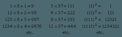
Number patterns and curiosities

Some groupings of natural numbers reveal remarkable patterns when you hit them with ordinary arithmetic. It affords pleasant pastimes. Take a look at this example:

The Hidden Math Behind Multigrades

It isn’t just about adding up a few integers. Multigrades are a specific breed of number play where two different sets of numbers share more than just their basic sum. They match up when you raise them to higher powers too.

“Identities between the sums of two sets of numbers and the sums of their squares or higher powers.”

Think of it as a mathematical mirage. You take Set A and Set B. Add the numbers in each. The total is identical. Now square every number in both sets. The sums of those squares are also identical. You can go even further—cubes, fourth powers, and beyond.

This isn’t random luck. It’s a structured identity. Mathematicians use this to explore how numbers relate beyond simple arithmetic. It’s a puzzle that requires precision. One wrong digit and the entire symmetry collapses.

Why do we care? Because these patterns reveal deep connections in number theory. They show that integers can behave in surprising, coordinated ways. It’s like finding two entirely different songs that somehow share the same rhythm and melody.

The study of multigrades continues to fascinate. It’s a niche corner of math that feels almost magical. And it all starts with a simple question: can two different groups of numbers truly be the same in multiple dimensions?

Building Multigrades from Scratch

Start with something trivial. A simple equality like 1 + 5 = 2 + 4. It’s barely worth noticing. Then add five to each term. The math holds. 6 + 10 = 7 + 9.

This is the seed. The easy method for forming a multigrade begins here.

But that’s just the setup. To get to a second-order multigrade, you have to flip the script. Switch the sides. Combine them.

It looks like this:

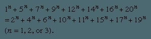
1 + 5 + 6 + 10 = 2 + 4 + 7 + 9

The numbers don’t lie. They balance.

Look at the math for a second. If you take a specific set of numbers, the sum of their first powers ($S_1$) lands exactly on 22. Add up their second powers ($S_2$), and that figure jumps to 156. It’s a tight little mathematical pocket.

But then you tweak it.

Take every single number in that set and just add 10 to the mix. Suddenly, you aren’t just playing with basic sums anymore. You have unlocked a third-order multigrade.

This isn’t just about arithmetic trivia. It’s about how shifting a baseline changes the structural integrity of a number sequence. By translating the entire set by a constant factor, you preserve the equality of the power sums across both sides while elevating the order of the identity.

The result? A more complex equation that holds up under the scrutiny of third-power calculations. The numbers change, but the balance remains. And sometimes, all it takes to unlock a deeper pattern is adding ten to every term.

Beyond Multigrades: The Weird World of Number Curiosities

If you thought you had seen it all with standard sum-powers equations, look closer. The math doesn’t stop at a few variables. It spirals.

Let’s look at the example again. S 1 sits at 84. S 2 jumps to 1,152. S 3? That’s 17,766.

You can keep going. Indefinitely. Building multigrades of successively higher orders. The structure holds.

Here is the trick: multiply or divide every term by the same number. The equality remains untouched. It is flexible.

Variations abound. You can find palindromic multigrades. These read the same backward and forward. Or maybe you prefer prime numbers. You can build multigrades composed entirely of them.

But there are other oddities lurking in the integers. Narcissistic numbers.

These are numbers that can be represented by some kind of mathematical manipulation of their digits. Take a whole number. An integer. Raise each digit to the n th power. Sum them up. If the result is the original number, you have found a perfect digital invariant.

Consider 153.

13 + 53 + 33 = 153.

It works. The digits power themselves and sum to their parent.

Then there is the recurring digital invariant. It loops.

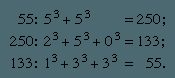
The world of recreational math loves a good party trick, and digital invariants are the life of the party. Joseph Madachy, in his book Mathematics on Vacation, points out that these aren’t just isolated curiosities. They come in variations that keep mathematicians entertained for hours.

The Power of Summed Digits

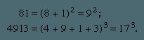
One specific type of curiosity stands out. It involves a number that equals the n th power of the sum of its digits.

Think of it this way. Take a number. Add up its digits. Raise that sum to a specific power. If the result is the original number again, you have found a match. It is a loop. A digital echo.

“A curiosity is exemplified by a number that is equal to the n th power of the sum of its digits.”

This isn’t just any random property. It defines a specific class of integers that behave unusually under basic arithmetic operations. The “n” here is the key variable. It determines the strength of the exponent. Change the power, and the number usually breaks the pattern. That’s what makes it a digital invariant. The sum stays constant relative to the transformation defined by n.

Madachy highlights this because it shows how simple rules—adding digits, then exponentiating—can lead to stable points. These numbers anchor themselves against the chaos of calculation. They are rare. But they exist. And once you find one, you start looking for others. The hunt becomes the game.

You’ve probably heard of automorphic numbers. They are integers whose squares end with the exact same digits as the original number. Take 25. Square it and you get 625. The last two digits? Still 25. Try 76. The square is 5776. Again, it ends in 76. These aren’t just random coincidences. They are mathematical quirks that feel almost mystical.

Then there are strobogrammatic numbers. These look identical when you rotate them 180 degrees. Think about 69. Flip it. It becomes 96. Wait, that’s not quite right for “reading the same.” Let’s look at 96 rotated. It looks like 96 upside down? No, actually, 6 becomes 9 and 9 becomes 6. So 69 rotated is 69? No, 69 rotated 180 degrees looks like 69. Yes. And 96 rotated looks like 96. Also 1001. Flip it. Still 1001. These properties suggest that numbers have hidden personalities.

The Four Nines Challenge

This leads us into the realm of digital problems. The most famous of these is the problem of the four nines. You might know it as the “four 9s” or “four 4s” depending on the digit. The goal is simple but deceptively hard. Express as large a sequence of integers as possible starting from 1. You must represent each integer using exactly four of the same digit.

But here is the catch. The answer depends entirely on the rules of operation you are allowed to use.

If you are just doing basic arithmetic, the sequence stops quickly. You need to get creative. Factorials? Square roots? Decimal points? Concatenation? Each allowed operation opens new doors.

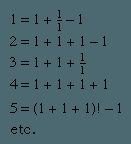
Consider the partial examples for four 1s. It starts easy.
1 = 1 + 1 – 1 – 1 (No, that’s 0).
1 = 1 * 1 * 1 * 1.
2 = 1 + 1 + 1 – 1.

The constraints force you to think laterally. Which operations are permitted? Can you use a double factorial? Can you concatenate two 1s to make 11? The specific rules change the entire landscape of the puzzle.

Why the Rules Matter

Different versions of this puzzle exist. Some allow only +, -, *, /. Others include exponents, logarithms, or the gamma function. The more tools you have, the higher the numbers you can reach. This isn’t just about math. It is about the boundaries of notation.

Strobogrammatic numbers and automorphic numbers are static curiosities. They sit there in the number line. The four nines puzzle is dynamic. It requires action. It requires you to bend the rules of representation.

There is a reason these puzzles persist. They appeal to the part of the brain that enjoys pattern recognition within strict constraints. It is a game of limitation. The more you restrict the digits, the more you must expand your understanding of what is possible.

Does the mysticism of automorphic numbers feel satisfying? Or is the active

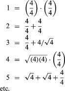
You think you’ve cracked the code on the four 4s? Think again.

The original list from M. Bicknell and V. Hoggatt’s 1964 Recreational Mathematics Magazine article was just the tip of the iceberg. They showed one way to hit sixty-four targets. But the real fun lies in the alternatives.

Take the number seven. The standard approach might use addition and square roots. But you can just as easily use factorials. Or division.

Consider this:

7 = 4 + √4 + 4/4

That works. But so does this:

7 = 4!/4 + 4/4

And here is another twist:

7 = 44/4 – 4

The factorial symbol (!) is the wildcard here. It turns a simple number into a product of all integers leading up to it. So 4! is just 4 × 3 × 2 × 1. That gives you 24. Suddenly, you have new tools in the box.

What Happens Without Factorials?

If you ban factorials from the ruleset, you don’t lose the game. You just shrink the board.

You can still express every integer from one to twenty-two using four 4s. It requires getting creative with decimals and roots.

Look at twenty-two. Without factorials, you lean on the decimal point and the square root.

22 = (4 + 4) / .4 + √4

The decimal .4 is essentially 0.4. Dividing 8 by 0.4 gives you 20. Add the square root of 4 (which is 2), and you hit the target. It’s ugly. It’s clever. It works.

But if you expand the rules again? The possibilities explode. You aren’t limited to basic algebra anymore. You can layer operations. You can chain them.

The Next Level: Sequential Integers

There is a sibling problem to the four 4s puzzle. It flips the script.

Instead of using the same digit four times, you use the first m positive integers. The rule is simple: m must be greater than three.

You use elementary algebra symbols. You arrange the numbers 1, 2, 3, and 4.

This shifts the challenge from repetition to sequence. You can’t just add 4s together. You have to weave 1, 2, 3, and 4 into a functional equation.

It’s a different kind of mental gymnastics. And it’s only getting started.

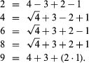
There are over 100 ways to arrange the digits one through nine to hit exactly 100. That is not even the hard part. These puzzles require brain power. They do not require advanced math.

The Origin of Cryptarithms

The term crypt-arithmetic arrived in 1931. It started with a multiplication problem in the Belgian journal Sphinx. That publication was known for its brain teasers.

“Crypt-arithmetic” was introduced in 1931, when the following multiplication problem appeared in the Belgian journal Sphinx

The problem looked simple. It was just letters representing numbers. Solving it felt like cracking a code. The ingenuity required is high. The actual arithmetic is minimal. You are looking for patterns. You are matching constraints.

These puzzles have many variations. Some ask for sums. Others demand products. The goal is always the same. Find the hidden number behind the letter. It is a game of logic. Not a test of calculation.

Cryptarithms are mathematical puzzles where digits are replaced by letters or symbols. Most involve basic operations like addition, subtraction, multiplication, or division. Solving them requires logic, not guessing.

The process starts with analysis. Take a simple example. You look at the partial products. If D × A equals D, then A must be 1. That’s a hard fact.

Next, look at C. If D × C and E × C both end in C, C is usually 5. Zero works if both digits are even. Five works if both are odd. Here, C = 5.

Now for D and E. They have to be odd. But not 9, because the partial products only have three digits. So they’re 3 or 7. Which is which?

Check B. If D × B is a single digit, B must be small. If E × B is two digits, E is larger. So E = 7 and D = 3.

B can’t be zero. That leaves 2. So B = 2.

Finish the math. F = 8. G = 6. H = 4. The answer is 125 × 37 = 4,625.

This breakdown comes from 150 Puzzles in Crypt-Arithmetic by Maxey Brooke. Dover published it in 1963. It’s still a classic for a reason.

The SEND + MORE = MONEY Breakdown

These puzzles are older than Brooke’s book. Sometimes they appear before records. Alphametics are a specific type. The letters form real words. One of the oldest and best-known is SEND + MORE = MONEY.

It’s a simple equation. But it’s deceptively complex.

S = 9. E = 5. N = 6. D = 7. M = 1. O = 0. R = 8. Y = 2.

9567 + 1085 = 10652.

Check the math. It works. Every letter has a unique digit. No leading zero. M can’t be zero. S can’t be zero. The constraints tighten quickly.

Why does this puzzle endure? It’s clean. It uses common words. It feels like a code. You’re not just doing arithmetic. You’re decoding a message.

Other alphametics exist. CROSS + ROSES = ARSENIC. EAT + THAT = CAKE. They vary in difficulty. Some are trivial. Others take hours. The logic is the same though. Find the anchors. A digit that forces another. A carry that breaks the pattern.

People still solve them today. Not just for the math. For the satisfaction. The moment the pieces click. The hidden word revealed. It’s a mental workout. Short. Sharp. Satisfying.

The puzzle doesn’t end with the answer. It ends with understanding. How the letters interact. How the numbers behave. It’s a tiny world. Self-contained. Logical.

And yet. You’ll see it again. In a magazine. On a forum. In a classroom. The same logic. Different words. Different numbers. Same thrill.

Is there a limit to how complex these

Standard rules for alphametics are strict. The first letter of any word cannot be zero. No two letters can stand for the same digit. Break these rules and you need a specific clue to justify the exception. Some puzzles are so dense they hold multiple solutions. Computers crunch through these complexities.

The Trap of False Logic

Mathematicians have obsessed over paradoxes and fallacies for centuries. A paradox stops you cold. The logic holds up. Every step is valid. Yet the conclusion is so bizarre you refuse to believe it. It’s counterintuitive. It feels wrong.

A fallacy is different. It’s a mistake. Improper reasoning leads to a result that is obviously absurd. The error usually breaks a core principle of math or logic. Beginners fall for it hard. They don’t see the hidden trap. Unless you know the rule being violated, the error stays invisible.

Then there are the sophisms. The error is intentional. Done on purpose. For a specific reason. But what if a flawed calculation accidentally lands on the right answer? That’s a howler. It’s the art of making the right mistake.

Infinity causes a lot of trouble. Limiting processes create paradoxes. Take the infinite series.

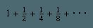
The Infinite Sum That Never Quite Touches 2

You’ve got a series that keeps climbing. The more terms you add to the pile, the higher the total gets. It’s a steady, relentless rise. But here is the catch. The sum never actually hits 2. It stays strictly below that ceiling.

It just gets closer. And closer. And closer.

Think of it like running toward a wall. You cover half the distance, then half of what’s left, then half again. You are always moving forward. You are always getting nearer to the target. But you never quite touch it. This is the behavior of a convergent series. Specifically, one bounded by 2.

“The sum always remains less than 2, although it approaches nearer and nearer to 2 as more terms are included.”

This isn’t just a math trick. It’s a fundamental concept in calculus. It’s about limits. We aren’t looking for the final number because there isn’t one. We’re looking for the behavior as the number of terms goes to infinity.

Why It Matters for Pop Culture Math

Okay, maybe you don’t care about series convergence. But this logic applies to everything. Think about streaming numbers. A show might gain more viewers every week. The growth slows down. It approaches a saturation point. But it never quite hits that theoretical maximum. It hovers just below.

Or think about box office totals. A movie grosses more each weekend. The rate of growth drops. The total sum inches toward a final number. But until the last ticket is sold, it’s always an estimate. A limit.

The same rule applies to celebrity followers. They gain more fans each day. But the account never truly stops growing until the person passes away or goes silent. Even then, the historical total is a snapshot. A moment in time.

The Other Series

On the other hand, the series…

Well, the text cuts off. But usually, in these comparisons, the “other series” is the divergent one. The one that doesn’t care about limits. The one that just keeps growing. Forever. No ceiling. No wall.

Just endless expansion.

Which is scarier? The thing you can never quite reach? Or the thing that never stops coming?

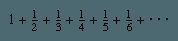
Math has always loved a good plot twist. You think you have it figured out? Think again. Take the series known as Divergent: It Has No Limit. If you keep adding terms, the sum doesn’t just grow. It explodes. It becomes larger than any value you can choose. It’s a runaway train with no brakes.

Then there is the even number paradox. It’s a head-scratcher that breaks your intuition.

There are just as many even natural numbers as there are even and odd numbers combined.

Think about that.

The set of even numbers is a subset of the total natural numbers. In our finite world, the whole is always greater than its parts. You can’t have 5 apples and have just as many apples if you only count the red ones. But infinity? Infinity doesn’t care about your rules.

This contradiction isn’t a bug. It’s a feature of infinite collections.

Since both are infinite, they are for both practical and mathematical purposes equal.

It feels wrong. It looks wrong. But mathematically, if you can pair every element in one set with a unique element in another, they are the same size. You can map the natural numbers (1, 2, 3…) to the even numbers (2, 4, 6…) one-to-one. No leftovers. No gaps.

The whole is not greater than its parts here. The parts are the whole.

This is where human logic hits a wall. We evolved to count berries and spot predators, not to navigate the abstract depths of endless sets. When you deal with an infinite number of objects, equality takes a backseat to correspondence.

So, is it a paradox? Technically. It contradicts the ancient notion that the whole is greater than any part. But it’s only a contradiction if you insist on applying finite rules to an infinite canvas.

Once you accept that infinity behaves differently, the “contradiction” disappears. It’s just a different kind of equality.

Why does this matter to you? It’s not just academic jargon. It’s the foundation of calculus, of understanding rates of change, of how we model the universe. Without grasping that some things don’t add up in the traditional sense, modern physics stays stuck in the mud.

But it’s still weird.

You can keep dividing a line in half forever. You’ll never reach the end. You’ll never finish. And yet, you get there.

How do you reconcile that with the way you move through the world? You don’t. You just accept the math and move on.

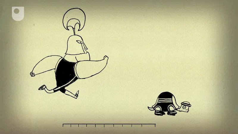
Zeno of Elea didn’t actually think Achilles could never catch the tortoise. He just loved a good logical trap.

Around 450 BCE, he whipped up four arguments designed to break your brain. The setup is simple. Achilles races a tortoise. The tortoise gets a head start. Zeno argues that Achilles can never overtake him. Why? Because before he reaches the spot where the tortoise was, the tortoise has moved to a new spot. And then another. And another. Infinite steps. No finish line.

It’s a sophism. A trick. Zeno knew it was flawed. His goal wasn’t to prove motion impossible. It was to expose flaws in how we think about space and time.

The other three paradoxes hit similar notes. The Dichotomy claims motion can’t even start. You have to cross half the distance first, then half of that, forever. The Arrow argues that at any single instant, a flying arrow is actually motionless. If time is made of instants, and it’s still in every instant, it never moves. Then there’s the Stadium, which messes with your sense of time intervals. It suggests a short duration equals a long one. Just to keep you off balance.

These weren’t just word games. They were probing the edges of limits and infinity. Concepts so slippery they stayed unresolved for millennia. It took until the 19th century for math to catch up. Rigorous analysis finally arrived. Transfinite number theory got a foundation. Only then could we properly explain why Zeno’s infinite steps don’t actually prevent Achilles from winning the race.

But let’s shift gears. Move from ancient Greece to your high school algebra class.

Common algebraic fallacies operate on similar principles of hidden traps. They usually break one or more of these basic assumptions:

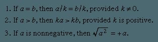
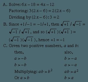
It starts with a simple contradiction. You think you’re doing algebra. You’re not. You’re building a house of cards in a hurricane.

Take variable a. And variable b. Standard stuff. But then the rules twist. Suddenly, a has to be bigger than b. And also smaller than b. At the same time. This isn’t just wrong. It’s impossible. It’s a violation of basic reality. You can’t be both above and below the line.

That’s the first example of a logic error. A clean, hard break.

Then there’s the second kind of mistake. The messy one. The “lucky boner.”

No, that’s not a typo. That’s a term. It refers to an illegal operation. You get lucky. You stumble into a result that looks right but is fundamentally broken. It’s a hack. A workaround that doesn’t hold water. You’re not solving the equation. You’re faking the solution.

And you’ll know it’s fake because it won’t survive scrutiny. The numbers won’t add up. The logic will collapse. Just like a can’t be both greater and less than b.

These aren’t just typos. They’re structural failures. You build on them, the whole thing comes down.

The Pythagorean obsession with number shapes

Numbers aren’t just abstract symbols. To the Pythagoreans, circa 500 BCE, they had personality. They had shape.

This fascination wasn’t new. Ancient Chinese scholars likely knew these concepts. By the 15th century, they appeared in arithmetic books. But the ancient Greeks took it further. They believed everything could be explained by numbers. And those numbers had specific characteristics.

This led to the discovery of polygonal numbers. Also known as figurate numbers, these represent counts arranged into geometric figures. It’s a concept that sounds simple today. But back then, it was a revelation.

Numbers were invested with specific characteristics and personalities.

Take the triangle. It’s the most basic shape. The first triangular number is 1. The second is 3. The third is 6. Then 10. Then 15. Then 21.

Visualize it.

Points or dots arranged in the shape of a triangle.

It’s not just a list. It’s a visual pattern.

But why did this matter so much to Pythagoras and his followers?

Because they saw the universe as mathematical. If you can map a number to a physical shape, you’ve found a piece of the truth. It wasn’t just about counting. It was about structure.

This idea sparked centuries of exploration. Mathematicians didn’t stop at triangles. They looked for squares. Pentagons. Hexagons. Each shape revealed new relationships.

The Pythagoreans recognized that numbers had “shapes.”

This insight changed how we think about arithmetic. It wasn’t just about addition and multiplication. It was about geometry.

And it started with dots.

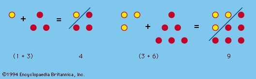
If you look closely at a sequence of triangular numbers—1, 3, 6, 10—you will find a hidden geometric pattern that explains why squares are so common in nature and math. The relationship isn’t arbitrary. It is structural.

Square numbers, which are the squares of natural numbers like 1, 4, 9, 16, and 25, have a visual representation. They can be arranged into perfect square arrays of dots. This visual proof is often shown in introductory geometry, but the deeper connection lies elsewhere.

The Triangle-to-Square Connection

The real magic happens when you combine adjacent triangular numbers. Take the first two triangular numbers: 1 and 3. Add them together. The result is 4. That is a square number.

Now try the next pair. The second triangular number is 3. The third is 6. Add them. You get 9. Another square.

This is not a coincidence. The sum of any two adjacent triangular numbers always equals a square number.

“The sum of any two adjacent triangular numbers is always a square number.”

This geometric truth explains why squares appear so often in counting systems. It is not just about squaring a variable. It is about stacking shapes. If you arrange dots in a triangle and then place another, slightly larger triangle next to it, they fit together perfectly to form a larger square.

This property links number theory directly to visual space. It turns abstract arithmetic into a physical puzzle. You do not need a calculator to see it. You only need to draw it.

And that is why we keep coming back to these basic shapes. They are the building blocks for everything else.

Why Oblong Numbers Matter in Pop Culture Math

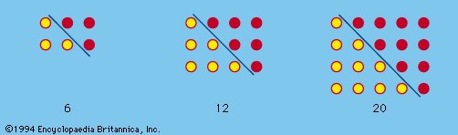
You don’t see oblong numbers mentioned in every movie script, but they’re hiding in plain sight whenever a film deals with grids, arrays, or even just basic geometry. Think of them as the rectangular cousins of triangular numbers. They’re not just abstract concepts. They are specific integers that represent dots arranged in a rectangle where one side is exactly one unit longer than the other.

The sequence starts small. 2, 6, 12, 20, 30. Simple enough. But look closer. Each number is the product of two consecutive integers. 1 times 2 equals 2. 2 times 3 is 6. 3 times 4 yields 12. It’s a pattern that repeats with mechanical precision.

“Oblong numbers are formed by doubling any triangular number.”

This relationship is key. If you take a triangular number—like 1, 3, 6, 10—and double it, you get an oblong number. 1 doubled is 2. 3 doubled is 6. 6 doubled is 12. The math holds up. It’s a direct link between two fundamental shapes in number theory.

Some might ask why this matters outside a textbook. It doesn’t. Not really. But it’s fun to know that 20 isn’t just a random age or a year. It’s 4 times 5. It’s also 2 plus 4 plus 6 plus 8. The sum of the first four even numbers. That’s the second way to build these figures. You can multiply consecutive pairs or stack even numbers. Both paths lead to the same oblong destination.

This isn’t just about dots on a page. It’s about structure. Rectangles everywhere—from the aspect ratio of a cinema screen to the layout of a spreadsheet—rely on this kind of proportional thinking. Oblong numbers are the mathematical backbone of that proportion. They’re the hidden order behind the chaos of everyday shapes.

The Geometry of Odd Numbers

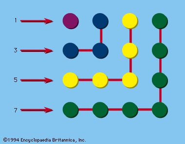
Think of a gnomon as a geometric L-shape. It isn’t just a random squiggle. It mirrors the right angle of a carpenter’s square. The Pythagoreans didn’t just use these shapes for decoration. They treated them as building blocks.

The math is surprisingly simple once you see the pattern.

Start with a small square. Add a gnomon. You get a bigger square. The numbers follow a strict rhythm. You can build squares by stacking these shapes onto smaller ones. This allowed them to deduce complex interrelationships without modern algebra.

Consider the sequence of squares.

• 1 squared plus 3 equals 2 squared
• 2 squared plus 5 equals 3 squared
• 3 squared plus 7 equals 4 squared

It’s a chain reaction. But there is another way to look at it.

You can sum consecutive odd numbers to reach a perfect square.

• 1 plus 3 equals 3 squared
• 1 plus 3 plus 5 equals 4 squared
• 1 plus 3 plus 5 plus 7 equals 5 squared
• 1 plus 3 plus 5 plus 7 plus 9 equals 6 squared

The list goes on. It’s elegant. It’s clean.

This specific property of gnomons in Pythagorean mathematics likely sparked the discovery of the most famous theorem in history. Pythagoras didn’t stumble upon the relationship between the sides of a right triangle by accident. He was contemplating square numbers.

He noticed that adding an odd square to an even square could form a third square. The visual proof was right there in the L-shapes.

a squared plus b squared equals c squared.

The geometry explained the algebra. Or rather, the geometry was the algebra. They didn’t have symbols for variables. They had shapes. And those shapes told a story about numbers.

Why did it matter so much? Because it linked addition to multiplication. It linked lines to areas. It turned abstract counting into tangible space.

The gnomon was the key. It unlocked the door to understanding how numbers grow. How they fit together. How they create structure out of chaos.

It’s strange to think that such a simple L-shape holds so much power. But then again, simplicity is often where the deepest truths hide.

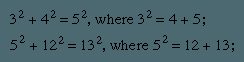
The math gets weirdly specific here. We are looking at a case where $a^2 + b^2 = c^2$, but with a catch: $a^2$ equals $b + c$. It’s a niche slice of Pythagorean triples. The Greeks didn’t just stop at right triangles though. They obsessed over shapes. Pentagonal numbers. Hexagonal numbers. They mapped geometric patterns directly to algebra. It wasn’t abstract art. It was arithmetic with edges.

These fall under the broader umbrella of figurate numbers. Polygonal numbers are just one subset. The list starts with simple arithmetic sequences, but the pattern holds.

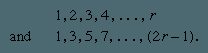
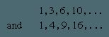
The sums of these series don’t yield simple arithmetic progressions. They build something more structured. You get polygonal numbers. Specifically triangular and square numbers. But the math doesn’t stop at two dimensions.

From Polygons to Pyramids

Add these sequences together again and you climb into three dimensions. The results are figurate numbers. We call them pyramidal numbers.

This isn’t just historical curiosity. These numbers connect directly to modern number theory. Even basic properties of integers can require heavy machinery to explain.

Take this rule. Every integer falls into one of three categories. It is:

1. A triangular number.
2. The sum of two triangular numbers.
3. The sum of three triangular numbers.

The proof is elegant but complex. Here is how it looks in practice.

“8 = 1 + 1 + 6”
“42 = 6 + 36”
“43 = 15 + 28”
“44 = 6 + 10 + 28”

Four equals six. Wait. No. Fourteen equals six plus eight. That is two triangles. But four four requires three. Six plus ten plus twenty eight.

Pythagorean Triples

Move from sums to squares. The Pythagorean theorem opens doors you didn’t know existed. A Pythagorean triple comes from the sides of a right triangle with integer lengths.

Find three positive integers a, b, and c where:

a ² + b ² = c ²

If those numbers share no common factor, they form a primitive Pythagorean triple. Relatively prime. That is the key constraint.

We need a way to generate them all. Not just find one or two. All of them.

There is a formula. It works for generating all primitive Pythagorean triples.

If m and n are positive integers with m > n, and m and n are relatively prime, and one is even while the other is odd, then:

a = m ² – n ²
b = 2m n
c = m² + n*²

Try m = 2, n = 1.

a = 4 – 1 = 3
b = 2(2)(1) = 4
c = 4 + 1 = 5

3, 4, 5. The classic triple.

Try m = 3, n = 2.

a = 9 – 4 = 5
b = 2(3)(2) = 12
c = 9 + 4 = 13

5, 12, 13.

It seems simple enough until you try to prove it covers every possible case without duplicates. The conditions on m and n are strict. They filter out the non-primitive sets. They ensure the primitive status.

Why do we care about the generators? Because once you have the generator, you have the structure. You can trace back to any triple.

The formula for generating these triples relies on picking two specific integers, p and q, and following a strict set of rules. It isn’t just about picking any two numbers. You have to be careful.

The first rule is that p and q must be relatively prime. That means they share no common factors other than one. The second rule is even more specific: they cannot be both even, and they cannot be both odd. This forces one to be even and the other to be odd. Finally, you must choose p to be larger than q.

When you hit all these marks, the math clicks into place.

Why Parity Matters in Triple Generation

This odd-even requirement is not arbitrary. If p and q were both odd, the resulting squares would create a sum that is divisible by 4, leading to a triple where all sides share a factor of 2. That breaks the “primitive” condition. The same happens if they are both even, since you can just divide out the 2s.

By forcing one even and one odd input, you ensure the output sides don’t share a common divisor. The result is a primitive Pythagorean triple.

Examples of Generated Triples

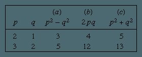
Choosing p and q appropriately yields classic sets. For instance, if you pick p = 2 and q = 1:

• The first side becomes $p^2 – q^2 = 3$
• The second side becomes $2pq = 4$
• The hypotenuse becomes $p^2 + q^2 = 5$

You get the 3-4-5 triangle. It’s the most basic one. Everyone knows it. But it works because 2 and 1 are coprime and of mixed parity.

Try p = 3 and q = 2.

• Side A: $9 – 4 = 5$
• Side B: $2(3)(2) = 12$
• Hypotenuse: $9 + 4 = 13$

That gives you 5-12-13. Another primitive set.

The pattern holds. You just need to find those coprime pairs with mixed parity and watch the geometry unfold.

You might think primitive Pythagorean triples are scattered randomly across the number line, but they aren’t. There’s only one instance where you get three consecutive integers that form such a triple. It’s the classic 3, 4, 5. That’s it.

Once you move past that single anomaly, the rules get interesting. Even in a standard primitive triple where a and b are the legs and c is the hypotenuse, specific modular arithmetic constraints always apply. You can count on it.

Divisibility by 3, 4, and 5

One of the legs, either a or b, will always be divisible by 3. Another leg will always be divisible by 4. And if you look at all three sides, one of them has to be divisible by 5. This isn’t just a coincidence for small numbers. It’s a structural rule.

Because of this, the product of the three sides (abc ) is always divisible by 60. It’s a clean, predictable pattern in a field that often feels chaotic.

The Number 7

Then there’s 7. It’s a bit more complicated. One of the following quantities must be divisible by 7:
* a
* b
* a + b
* a – b

It’s not always the sides themselves. Sometimes it’s the sum or the difference. But 7 always shows up in one of those forms.

There’s also a formula that generates valid Pythagorean triples for any integer n. If you plug in a number, you get:
1. 2n + 1
2. 2n ² + 2n
3. 2n ² + 2n + 1

These always form a right triangle. It’s a reliable way to generate triples without memorizing lists.

The Ancient Greek Constraints

The Greeks knew some of this long before we had calculators. They knew the hypotenuse of a primitive triple is always an odd integer. They didn’t have the full modern proof, but they had the intuition.

Today, we have a precise condition. An odd integer R serves as the hypotenuse of a primitive triple if and only if every prime factor of R is of the form 4k + 1. This restricts which odd numbers can even appear in that position. It eliminates half the odds right out of the gate.

Perfect Numbers and Mersenne Primes

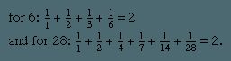
Most integers are either abundant or deficient. The distinction is simple. An abundant number has proper divisors (excluding itself) that sum to more than the number. A deficient number’s proper divisors sum to less.

A perfect number sits right in the middle. It equals the sum of its proper divisors.

Take 24. Its divisors (1, 2, 3, 4, 6, 8, 12) add up to 36. It’s abundant.
Take 32. Its proper divisors sum to 31. It’s deficient.

Then you have 6. 1 + 2 + 3 = 6. Perfect.
Then 28. 1 + 2 + 4 + 7 + 14 = 28. Also perfect.

The next two are 496 and 8,128. The ancients knew the first four. They didn’t know if the list went on forever, or if the next one was a million digits long.

Euclid and Euler

Euclid made a guess. He suggested that numbers of the form 2n -1(2n -1) are perfect, provided that 2n -1 is prime. He was right about the generation, but he didn’t prove it was the only way.

That proof came much later. In the 18th century, Leonhard Euler showed that every even perfect number must fit Euclid’s formula. So if you’re looking for an even perfect number, you only need to look at Mersenne primes.

A Mersenne number is any number of the form 2n -1, named after Marin Mersenne. These can be prime or composite. For 2n -1 to be prime, n itself must be prime. It’s a necessary condition, though not sufficient. Just because n is prime doesn’t mean 2n -1 is. But if 2n -1 is prime, n has to be.

This creates a one-to-one correspondence. Every Mersenne prime yields an even perfect number. Every even perfect number comes from a Mersenne prime.

Finding the Giants

Until the computer age, finding these was a manual grind. Only 12 perfect numbers were known for a long time. Then Édouard Lucas gave us a primality test for Mersenne numbers in 1876.

Raphael M. Robinson took that test and ran it on early electronic digital computers. By 1952, he had found Mersenne primes for n values of 521, 607,

The Rabbit Problem That Started It All

It’s easy to forget that the Fibonacci sequence didn’t start in a computer science classroom. It began with a book. In 1202, Leonardo of Pisa—better known by his nickname, Fibonacci—published Liber abaci. This wasn’t just some dry math manual. It was a game-changer for European commerce, introducing Hindu-Arabic numerals to a continent still stuck on Roman numbers. But tucked inside that serious financial text was a silly little riddle about breeding rabbits.

The question was simple enough to explain over dinner. Imagine you start with one single pair of rabbits. Every month, that pair produces a new pair. Here’s the catch: the newborns don’t start breeding until they are two months old. So, in the first month, you have one pair. In the second, you have the original pair plus their babies. In the third, the original pair has another litter, and the first babies are now mature enough to have their own.

Do the math. It’s not hard. You get a specific string of numbers that keeps popping up in nature, code, and art.

How the Sequence Unfolds

Let’s look at the progression. It’s recursive, which is a fancy way of saying each number is the sum of the two before it.

• Month 1: 1 pair (the original)
• Month 2: 2 pairs (the original plus the first offspring)
• Month 3: 3 pairs (original, first offspring, second offspring)
• Month 4: 5 pairs

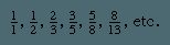
The sequence goes 1, 1, 2, 3, 5, 8, 13, 21, and so on. It’s clean. It’s logical. And it’s everywhere once you know where to look.

The Infinite Properties of Fibonacci Numbers

That second row? It’s the opening act of the sequence we now call Fibonacci’s. Each number after the first two is just the sum of the two before it. Simple math. x _n = x _n−1 + x _n−2. But nobody knew this rule was the key until roughly 1600.

The real explosion of interest came later. Specifically, the middle decades of the 20th century. Researchers dug into the properties of these numbers with a vigor that produced a mountain of literature. And it feels like the well is bottomless. The identities keep coming. Take this one for instance: x _n+1 · x _n−1 = x _n ² + (−1)ⁿ. It’s elegant. It’s persistent.

Then there’s Édouard Lucas. He had his own formula for generating these same numbers. A different angle on the same infinite puzzle.

The Math Behind the Magic Ratio

It starts with a number that refuses to be simple. The golden ratio, Phi (Φ), is roughly 1.618. Its reciprocal is 0.618. Both come from the roots of x ² − x − 1 = 0. This equation traces back to Luca Pacioli. A 15th-century Italian mathematician. He called it the Divine Proportion. The formula is a /b = b /(a + b ). When a is smaller than b. Set x to b /a and you get there.

It’s about dividing a line. Split it so the smaller part relates to the larger one exactly as the larger part relates to the whole. Ancient designers knew this. Modern architects use it too. A rectangle with sides in a 3:5 ratio feels right. Or 8:5. It’s aesthetically pleasing. Most pleasing, some say.

Powers of Phi

Raise Phi to successive powers. The sequence unfolds. It begins with specific numbers that echo the ratio itself.

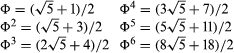
You might not expect a pop culture reference when looking at radicals, but there’s a hidden pattern in the square root of five. It’s not magic. It’s just math being math.

The coefficients in this sequence are the famous Fibonacci numbers. You know them. One, one, two, three, five, eight. They roll out like a heartbeat.

Look closer at the parentheses. The second terms follow a different rhythm. The Lucas sequence. It starts with one, three. Then four, seven, eleven, eighteen. It feels familiar. It is.

The Lucas sequence shares the same recursive heartbeat as Fibonacci. Each number is the sum of the two before it. The formula is simple. $x_n = x_{n-1} + x_{n-2}$.

It’s a neat trick. A mathematical Easter egg for anyone who likes patterns. The next time you see √5, think of the numbers hiding in the decimals. They’re there, waiting to be counted.

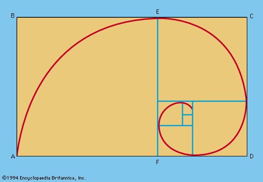
Start with a golden rectangle labeled ABCD. Chop off a square named ABEF. What’s left? Rectangle ECDF. It’s another golden rectangle. Same proportions. Different size. If you keep this up, the squares get smaller. The corners align. Draw circular arcs through them. The result isn’t a perfect circle. It’s a logarithmic spiral.

Nature loves this shape. You see it in nautilus shells. You see it in hurricanes. The math behind it is clean. The equation r = k Θ governs this curve in polar coordinates. The constant k is defined as Φ²/π. Phi squared divided by pi. It’s a precise relationship between growth and angle.

But the geometry isn’t just on paper. It’s in the garden. Fibonacci numbers explain phyllotaxis. That’s the fancy term for how plants arrange their parts. Look at a pinecone. Count the whorls. Look at a pineapple. The spirals intersect in Fibonacci numbers. Sunflower heads? Same thing. The petals don’t just grow randomly. They follow a sequence.

Why Plants Follow Fibonacci Rules

This isn’t coincidence. It’s efficiency. The specific sequence of fractions mentioned earlier helps seeds pack tightly. It ensures maximum exposure to light. Branches on some stems follow this same logic. They avoid shading each other. The plant optimizes its structure.

The spiral seen in Figure 4 approximates that natural growth. It’s an approximation because nature is messy. Biology doesn’t follow lines. It follows trends. The golden ratio appears in the spacing of leaves. It appears in the arrangement of seeds. It’s a pattern repeated across species.

Some might argue it’s just visual appeal. But the math holds up. The logarithmic spiral allows for expansion without changing shape. A leaf grows. It doesn’t distort. It scales. The Fibonacci sequence provides the integer steps for this scaling. It’s discrete growth in a continuous world.

The Connection Between Math and Biology

How does a seed know to grow in a spiral? It doesn’t. The physics of cell division favors these angles. The divergence angle approaches the golden angle. This minimizes overlap. It maximizes space. The result looks like a Fibonacci spiral. It is one.

You don’t need a degree in botany to spot it. Just look at the next pineapple you buy. Or the next sunflower. The numbers are there. Embedded in the structure. The golden rectangle is just the geometric abstraction. The plant is the physical reality. They are two sides of the same coin. One drawn with a compass. One grown in the soil. Both follow the same underlying rule.

Optical illusions aren’t just parlor tricks. They’re mathematical puzzles disguised as visual noise. The math behind them often relies on basic geometric principles. Specifically, the proportionality between the areas of similar figures and the squares of their linear dimensions. But it’s not all equations. There’s a physiological layer here. Your brain perceives relative lengths more accurately than relative areas. That gap in perception is where the illusion lives.

We’re talking about unorthodox perspective. Distorted angles. Deceptive shading. When you juxtapose colors in unusual ways, you trigger chromatic aberration. Afterimages follow. For a deeper dive into these mechanisms, you’d look up entries on illusion and hallucination. But the geometry gets weirder when you stop looking at static images and start looking at logical traps.

The Geometry of Lying

There are famous “proofs” in geometry that claim to show absurdities. They’re fallacies. And they’re seductive because they follow a logical structure, just with a fatal flaw.

Take the claim that every triangle is isosceles. It sounds wrong. It is wrong. Yet, some “proofs” convince you otherwise. Then there’s the assertion that every angle is a right angle. Or the idea that if you have a quadrilateral ABCD where side AB equals side CD, then AD must be parallel to BC. It’s false. You can construct a shape that fits the description without being a parallelogram. The most outrageous one claims every point in the interior of a circle lies on the circle itself.

How do these fallacies work? They don’t use magic. They use subtle errors.

The explanations for these bogus proofs usually boil down to a few recurring tricks. First, there’s faulty construction. The diagram is drawn slightly off, hiding the contradiction. Second, it’s a violation of logical principles. A common one is assuming the truth of a converse. If A implies B, that doesn’t mean B implies A. Confusing partial inverses or converses is a classic trap.

Sometimes, it’s a misinterpretation of a definition. The proof ignores “necessary and sufficient” conditions. It takes a condition that is required but not enough to prove the whole statement. And then there’s the human element. Too much dependence on diagrams and intuition. We trust our eyes over the logic. We get trapped by limiting processes and deceptive appearances. The brain sees what it expects to see.

When Shapes Have No Exit

This leads directly to impossible figures. These aren’t just optical tricks where lines cross. They are structures that cannot exist in three-dimensional space.

Think of the Penrose triangle. Three rods form a triangle. Each corner looks like a standard 90-degree joint. Put them together, and they loop. Your brain tries to resolve the depth cues. It assigns a front and a back to each edge. But the edges don’t connect. The figure demands a topology that breaks the rules of Euclidean geometry.

These recreations are topological nightmares. They force the eye to follow a continuous line that, if traced in real space, would have to pass through itself or bend in ways that defy physical constraints. Artists and mathematicians use them to highlight the limits of perceptual interpretation. They show that your brain is a prediction machine, not a camera. It fills

The Trap of Impossible Geometry

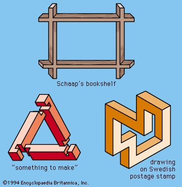
Look at Figure 5. Your brain wants to accept it. It sees plausible 3D objects. Solid. Real. But lean in closer and the illusion shatters. These drawings lie. They are built on faulty perspective, weird juxtapositions, or straight-up psychological tricks. You can’t build them. They don’t exist in space.

These are undecidable figures.

Oscar Reutersvard didn’t just dabble in visual paradoxes. He made them his thing. The Swedish artist turned these impossible shapes into the main event on a set of postage stamps. It was early. It was bold. And it proved that a postage stamp could be a gateway to a geometry that refuses to work.

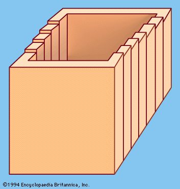
The Infinite Staircase and the Logic of Paradox

It started in 1958. L.S. Penrose, a British geneticist, and his son Roger Penrose, a mathematical physicist, introduced the world to strange loops. They weren’t just visual tricks. They were undecidable figures.

Take the Penrose square stairway. You can walk it in either direction forever. You never get higher. You never get lower. It’s an endless cycle. M.C. Escher took this concept and ran with it. His 1960 lithograph Ascending and Descending features monks walking this impossible path. Waterfall (1961) shows water defying gravity, looping back on itself. These aren’t just art. They are visual proofs of logical paradoxes.

Strange loops touch on infinity. They mirror self-referential statements like that of Epimenides. The philosopher claimed all Cretans were liars. If he was right, he was lying. If he was lying, he was right. The loop closes. The logic breaks.

When Curves Break the Rules

Mathematics has its own version of this madness. Pathological curves.

A standard continuous curve behaves. It has tangents. It has defined curvature. Pathological curves do not. They lack basic properties. Their tangent might be undefined at every single point. You can trace them. You can measure the area they enclose. That area is finite. The length? Infinite.

These aren’t optical illusions. They are real mathematical objects. They arise as limits of series of geometric constructions. The numbers converge. The shapes don’t quite fit. Their length approaches a limit. The area approaches another. But the object itself? It’s a paradox.

“Their idiosyncrasies constitute paradoxes rather than optical illusions or fallacies.”

This is where math stops being intuitive. You draw a line. It gets infinitely jagged. It stays in a small box. It has no slope anywhere. It’s a curve that refuses to be a curve.

We see this in the Penrose steps. We see it in Escher’s prisons. We see it in the math that underpins them. The infinite length within a finite space. The direction that leads nowhere. It’s not a mistake. It’s a feature.

The question isn’t how to fix it. It’s what happens when you accept the loop. Do you keep walking? Do you stop trying to find the end?

The curve continues.

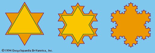
The Geometry of Infinite Perimeter and Finite Space

Take the Koch snowflake. Start with a simple equilateral triangle. Trisect each side. Replace that middle third with two sides of a smaller equilateral triangle that points outward. Do it again. And again. The process repeats infinitely. The first two steps are visible in Figure 7, showing how the shape gets bumpier, sharper, more complex with every iteration.

Here is the twist. The perimeter grows without limit. It goes to infinity. Yet the area it encloses stays finite. It approaches a specific ceiling. That upper bound is exactly 8/5 the area of the original triangle.

Think about that. You have an infinitely long boundary wrapping around a finite amount of space. It defies the intuition that longer lines mean more area. The Koch curve proves them wrong.

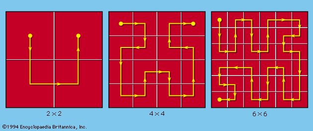
Filling space with a line that shouldn’t fit

It defies basic geometry. A curve is one-dimensional. It has length but no width. It shouldn’t be able to cover a two-dimensional area. Yet the construction in Figure 8 proves otherwise. If you keep going through the stages. The final result hits every single point in the square.

This isn’t a trick. The math holds up. The curve becomes space-filling.

From squares to cubes

You can stretch this logic further. It isn’t limited to flat surfaces. By applying the same reasoning. The curve can fill an entire cube. Three dimensions. One continuous line. It sounds impossible until you see the math work.

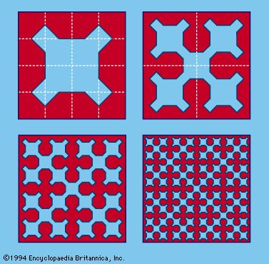
The Sierpinski curve is a weird beast. It starts as a simple square, but if you push the construction process far enough, it becomes something else entirely. It contains every single point inside that square. It forms a closed loop.

Here is the catch. Keep going. Indefinitely.

The length of the curve shoots toward infinity. It never stops growing. Yet, the area it encloses settles at exactly five-twelfths of the square’s total area. It’s a paradox of geometry.

“As the process of forming the curve is continued indefinitely, the length of the curve approaches infinity, while the area enclosed by it approaches 5/12 that of the square.”

Then there is the fractal curve. A loose definition works fine here. It’s a shape that keeps its irregular pattern no matter how much you zoom in. Think of von Koch’s snowflake. That’s the classic example.

Watch what happens at each stage of building it. The perimeter doesn’t just get bigger. It grows by a specific ratio. Four to three.

Benoit Mandelbrot changed the game in the 1950s. He didn’t like the old idea of dimension. He wanted a new symbol. D.

He treated dimension as a power. What power do you raise 3 to, so it equals 4? That’s the question. The answer isn’t a whole number. It’s log 4 divided by log 3. Roughly 1.26.

That is the dimension of the snowflake. It’s not a line. It’s not a plane. It sits somewhere in between.

Mandelbrot and his peers started looking at these “pathological” curves. They were obsessed with self-similarity. But they didn’t just stare at math. They looked at the world.

Random fluctuations in nature create statistical self-similarity. Mandelbrot’s techniques helped decode this. It works for fluid mechanics. Geomorphology. Human physiology. Economics. Linguistics.

Take Brownian movement. Look at microscopic surfaces. See the vascular networks in your body. Check the shapes of polymer molecules.

All of these are fractals. They share that same rough, repeating texture.

Mazes

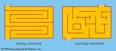
Solving the unsolvable

Put your hand on the wall. Keep it there. If a maze has only one entrance and one exit, this simple rule guarantees you will find the way out. It might not be the fastest route. You could take a detour. But you will get there.

What if the goal is tucked inside the labyrinth? The same hand-on-wall trick works. There is one catch. No closed circuits. If the maze contains a loop—a route that circles back to the start—the method fails. You will just spin in circles.

Mathematicians call a maze with no loops “simply connected.” If it has loops, it is “multiply connected.” To navigate these complex structures, you need a better plan.

Designate every junction as a node. Label paths as “new” or “old.” Here is how you thread the maze without getting lost:

• Never walk a path more than twice.
• Hit a new node? Pick a direction.
• Hit an old node or a dead end via a new path? Turn around and go back the way you came.
• Hit an old node via an old path? Try a new path. If none exist, take another old one.

People don’t play with paper mazes as much as they used to. The thrill has faded. But two modern fields still rely on them. Psychology uses them to study learning behavior. Communications technology uses them to improve computer design.

Cutting shapes into pieces

Geometric dissections are different. They involve cutting figures into pieces that can be rearranged. Take a rectangle. Cut it up. Reassemble the pieces into a square. Do it the other way around too.

Interest in this math puzzle started near the end of the 18th century. Montucla highlighted the problem. As it grew popular, the focus shifted. It wasn’t just about rectangles and squares anymore. It was about any polygon. How do you dissect a shape with n sides into a different shape with equal area?

By the early 20th century, the question changed again. It wasn’t enough to just do it. You had to find the minimum number of pieces required. Efficiency mattered.

A comprehensive theory emerged around 1960. It defined “equidecomposable” figures. Two polygons are equidecomposable if you can cut one into a finite number of pieces and rearrange them to form the other. They must have equal areas. Obviously.

The converse theorem is even stronger. If two polygons have equal areas, they are equidecomposable. Period.

There is also the method of complementation. Add congruent parts to two figures. Make the new figures congruent. These are “equicomplementable.” They also have equal areas.

The theory expanded. Researchers explored how equidecomposability relates to motion. Translations. Central symmetry. Groups of motion in general. The studies eventually reached polyhedra. 3D shapes. Much harder questions. Still being answered.

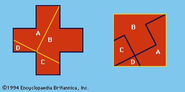
The Mechanics of the Greek Cross

Practical application demands more than just theory. Turning a Greek cross into a square isn’t a simple fold. You need ingenious procedures to make it work. The geometry gets tricky fast.

H. Lindgren documented some of these specific methods. His work is the go-to reference for anyone actually trying to solve this puzzle. You can find the details in the Bibliography. It’s not about guessing. It’s about following the steps that actually hold together.

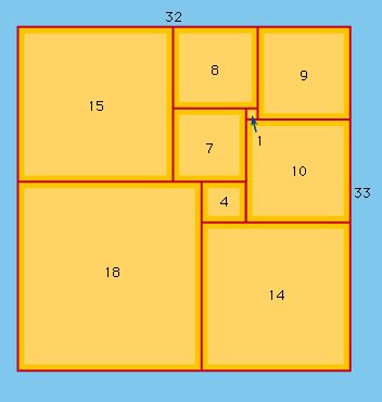
Squaring the Square: A Geometric Puzzle Solved

Forget the dusty textbooks. The idea that you couldn’t split a square into smaller, non-identical squares was once a stubborn myth. It wasn’t a lack of trying. Mathematicians stared at the blank page for decades. The solution didn’t come from compass and straightedge. It came from network theory.

This is squared rectangles. A rectangle dissected into a finite number of squares. If none of those squares are the same size, it’s perfect. The order? Just the count of those squares.

Here’s the kicker. There are no perfect rectangles with fewer than nine squares. Zero. Not one. But at order nine? Exactly two exist. One of them is shown in Figure 12. The dissection of a square into unequal squares, deemed impossible as early as 1907, was first reported in 1939.

It’s not magic. It’s topology.

How Graphs Solve Geometric Puzzles

The word graph trips people up. You picture a line chart. A stock ticker. A curve of analytic geometry. Wrong. Or at least, incomplete.

In puzzles, a graph is simpler. Points and lines connecting them. Linear graphs. Little more. And yet, these crude structures solved a problem that stumped geometers for over thirty years.

Why does this matter? Because it shows how abstract networks map onto physical space. You take a rectangle. You force squares into it. You track the connections. The graph reveals the hidden symmetry.

It’s not just about pretty shapes. It’s about logic. Pure, unadulterated logic.

“The dissection of a square into unequal squares, deemed impossible as early as 1907, was first reported in 1939.”

Three decades of dead ends. Then, a breakthrough. Not because someone got smarter. But because they stopped looking at the squares and started looking at the lines between them.

The graph doesn’t care about angles. It cares about connections. That’s the secret.

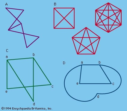
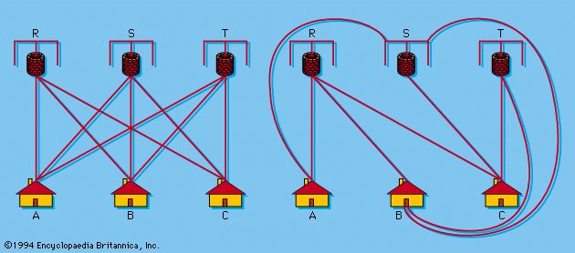
Graph Theory Basics: From Complete Graphs to Planar Puzzles

A finite set of points joined by lines forms a graph. Those points are vertices. The lines connecting them are edges. When every single vertex connects to every other vertex, you get a complete graph. But not all graphs are that simple.

Consider planar graphs. These are figures where edges don’t cross each other, except at the vertices themselves. The lines don’t have to be straight. You can curve them. This flexibility allows a nonplanar graph to be redrawn as an isomorphic planar graph, as seen in standard geometric illustrations.

The edges of a graph need not be straight lines. This distinction matters. It means a messy, crossing-heavy diagram might actually be planar if you just pull the lines apart.

The Three Wells Problem and Jordan’s Insight

Here is a classic puzzle. The “three wells” problem. Three houses. Three wells. You need paths from each house to each well. Total of nine paths. The rule? No path can cross another. It is impossible.

The proof relies on the Jordan curve theorem. A closed continuous curve splits a plane into an interior and an exterior. Any line connecting a point inside to a point outside must cut through the curve. This topological reality kills the three-wells puzzle.

Planar graphs aren’t just for puzzles. They are useful in designing electrical networks. Circuit boards often rely on planar principles to avoid short circuits and manage connectivity.

Connected Graphs and Paths

A connected graph is straightforward. Every vertex connects to every other vertex via an arc. An arc is just an unbroken sequence of edges.

There is also a path. A path travels across the graph without passing over the same edge twice. You can visit a vertex multiple times. Just don’t reuse the edge. It’s a specific type of traversal.

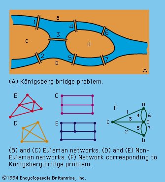
The roots of modern graph theory trace back to an 18th-century puzzle that seems simple enough for any casual walker to solve but turned out to be mathematically profound. It started with Leonhard Euler and the infamous Königsberg bridge problem. For decades after, the field was dominated by a specific type of route known as an Eulerian path. This is a figure you can draw without lifting your pencil or retracing any line.

The setting was the city of Königsberg, now known as Kaliningrad. The geography was messy. The Pregel River split into branches and surrounded an island. Seven bridges connected the various landmasses. The challenge posed to citizens was deceptively straightforward. Could someone leave their house, take a walk across these bridges, and return home having crossed each one exactly once?

Euler proved it was impossible. He didn’t just say “no.” He gave the world a new way to look at networks.

The rules of the network

Euler’s logic applies to any closed network, not just rivers and bridges. The solution lies in the points where lines meet.

• The number of even points—nodes where an even number of edges connect—is irrelevant to the path’s validity.
• The number of odd points—where an odd number of edges meet—must always be even. This holds true even if there are zero odd points.
• If there are no odd points, you can start anywhere and finish at the same spot.
• If there are exactly two odd points, you must start at one odd point and end at the other.
• If there are more than two odd points, a single continuous path is impossible. A network with $2n$ odd points can be traced in $n$ separate paths.

Why the bridges failed

Look at Figure 15F. It maps the Königsberg situation. The points represent the land areas. The edges represent the seven bridges.

The network has four odd points. That means you’d need four separate paths to trace it perfectly. Since people want a single continuous walk, the puzzle is unsolvable.

Other figures in the same set tell different stories. Figures 15B and 15C work. They follow Euler’s principles. You can traverse them using Eulerian paths. Figures 15D and 15E do not work. They break the rules of odd and even points.

The lesson stuck. We stopped looking at the curves and started looking at the connections.

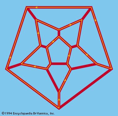
You might think network puzzles are just brain teasers, but they’re really about combining or arranging points in space. It’s older than you’d think.

Sir William Rowan Hamilton, an Irish mathematician, cooked one up in 1859. The challenge? Find a route along the edges of a regular dodecahedron. You had to pass through every point exactly once. No repeats. No shortcuts.

Later, people made it easier to play. They swapped the 3D shape for a flat graph with 30 edges. Same logic, less cardboard folding.

This is what we call a Hamilton circuit. It hits every vertex once. It doesn’t cover every edge, though. At each intersection, there are three edges. The circuit only uses two of them. The heavy lines in Figure 16 show one such path. There are plenty of others.

Graph theory and real-world chaos

Graph theory isn’t just for paper folding. It solves combinatorial headaches.

Think about connecting cities by rail. Or laying telephone lines. You need a network that works. Graph theory helps plan that.

It also handles traffic. It orders round-robin tournaments so every team plays every other team. It matches jobs to applicants. It’s the skeleton key for arrangement problems.

The four-colour map problem

Cartographers knew something mathematicians argued over for a century.

No map needs more than four colors. You can shade any region as long as adjacent areas differ. Simple rule. Hard proof.

In 1852, someone framed the “four-colour map problem.” Could you build a planar map that required five?

Mathematicians attacked it for years. They failed.

Then, in 1976, the University of Illinois team dropped the hammer. They proved four colors are enough.

Here’s the kicker. It was the first major proof to rely heavily on a computer. They ran over 1,000 hours of calculations. The diagrams came from the machine. Some mathematicians hated it. They said it wasn’t “human” enough. But it worked.

You can ask similar questions for other surfaces.

Maps on a torus (a donut shape) need seven colors. No more. No less.

The magic of flexagons

A flexagon is a polygon made from paper or foil. It looks like a flat strip until you flex it.

Then it changes faces.

They were first discussed in 1939. Now they’re a staple of math recs.

The trihexaflexagon is the simplest version.

Here is how you make one:
1. Cut a strip of material.
2. Mark off 10 equilateral triangles.
3. Fold it appropriately several times.
4. Glue the last triangle to the reverse side of the first.

Flex it. One face disappears. Another takes its place. It’s simple. It’s weird. It works.

Manipulative recreations

These aren’t just games. They’re models of how we structure space.

The origins of arrangement puzzles trace back to Lucas’ Puzzle. Picture a row of seven squares. The left three hold black counters. The right three hold white ones. The center square sits empty. Your goal: swap them. Black moves right. White moves left. You can slide into an adjacent empty spot or jump over an opponent’s piece. For n counters of each color, the move count is n (n + 2).

Scale it up. Or shrink it. The math holds.

There’s a sibling puzzle with eight numbered counters on nine spaces. Reverse the order. Only single moves and jumps allowed. No shortcuts.

Then there are the two-player games. Tic-tac-toe is the baseline. But the variations get spicy. Consider a version where each player starts with three counters. The board is a 3 × 3 grid. You place them one by one. You can’t use the center spot initially. If nobody gets three in a row after placement, you start moving. Adjacent squares only. Horizontal or vertical.

Win by forming a line.

Take it to a 4 × 4 board. Four counters each. Sometimes diagonals count. Try a 5 × 5 pattern. Or look across the Atlantic to Europe, where “mill” or nine men’s morris reigns. Three concentric squares. Eight transversals. Connect three to remove an opponent’s piece. It’s about blocking, not just aligning.

The geometry of connection

Hex is different. It’s not about lines. It’s about chains.

Piet Hein invented it in Denmark in 1942. The board is a diamond of tessellated hexagons. Usually 11 across each edge. “Tessellated” just means fitted together like tiles. No gaps. Two opposite edges are “white.” The other two are “black.”

Players alternate placing counters. The objective? Build an unbroken chain from your side to the other. White goes top to bottom. Black goes side to side.

The game never draws. Why? Because you can’t block your opponent without completing your own chain first. One path cuts the board. The game ends immediately.

John Nash invented it independently in the US in 1948. Years later, it hit the market as Hex.

Strategy here isn’t about simple alignment. It’s topological. It’s about control.

The queen’s dilemma

Chessboards offer their own mathematical headaches. The most famous? Place eight queens on a standard board. None can attack any other. C.F. Gauss worked on this around 1850. He wasn’t the only one obsessed.

Then there’s the knight’s tour. A closed tour. Start at a square. Visit every other square exactly once. End where you started. The math behind this is tangled with magic squares. Patterns within patterns.

Other problems dig into piece value. How many bishops can you fit without them taking each other? What’s the minimum number of knights needed to checkmate every square on the board?

Try placing 16 queens. No three in a straight line. Even that’s not trivial.

The Fifteen Puzzle

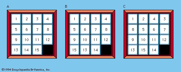
Sam Loyd the elder loved to claim he invented the Fifteen Puzzle around 1878. Modern scholars disagree. They found earlier inventors. The puzzle also went by other names. Boss Puzzle. Gem Puzzle. Mystic Square. It spread across Europe with terrifying speed. The setup is simple enough to confuse you. A shallow square tray. Fifteen small numbered counters. One empty square. You start with the numbers in random order. The blank space sits in the lower right. The goal? Rearrange the pieces into numerical order. You can only slide them. The blank space must end up back where it started. That’s the trick.

The sheer scale of the problem might make your head spin. There are more than 20 billion billion possible arrangements of the pieces. Including that blank space. In 1879, two American mathematicians proved something wild. Only half of those initial arrangements can actually be solved. That’s about 10 billion billion. The rest are dead ends.

The math behind this is elegant and slightly cruel. Think about the path any single number takes. As long as it ends up in the lower right corner, it passes through an even number of boxes. It’s a parity thing.

In the solved state, every number is larger than the ones before it. You read left to right. Top to bottom. No number precedes a smaller number. In any other arrangement, at least one number breaks this rule. This is called an inversion.

Take the sequence 9, 5, 3, 4. The 9 comes before three smaller numbers. The 5 comes before two smaller numbers. That’s five inversions total. It’s an odd number. If the total count of inversions in any given layout is even, the puzzle is solvable. Bring the squares back to normal. If the count is odd, you’re screwed. The puzzle has no solution.

Figure 17B has two inversions. Solvable. Figure 17C has five. Impossible. Theoretically, you can stretch this logic to any tray size. An m by n grid. With mn minus one numbered counters. The math still holds.

The Tower of Hanoi

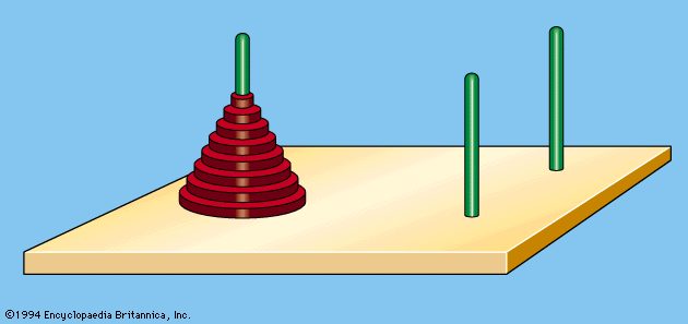
Edouard Lucas didn’t just invent a puzzle in 1883. He handed us a mathematical nightmare wrapped in wood.

French mathematician. Toy store staple. Three pegs. Eight disks.

It’s the Tower of Hanoi. Or at least, that’s who we’ve always blamed. Lucas gets the credit, though historians squabble over whether he actually created it or just popularized an older riddle. Doesn’t matter. The thing is everywhere. Plastic versions clutter shelves. Wooden ones sit on office desks. The rules are simple enough to explain in thirty seconds.

Place eight disks on one peg. Largest on bottom. Smallest on top. No big disk ever rests on a small one. Move the whole stack to another peg.

That’s it.

Except it isn’t.

The math hits you like a truck. For n disks, you need exactly $2^n – 1$ moves.

Eight disks? That’s $2^8 – 1$. 255 moves. Manageable. A bit tedious. A good test of patience.

But imagine the original legend.

A tower with sixty-four disks.

The number isn’t just big. It’s cosmically, terrifyingly big. $2^{64} – 1$.

18,446,744,073,709,551,615.

Try saying that out loud. It takes longer than a human lifespan to speak it. Now imagine making one move per second.

You’d be there for about 585 billion years.

The universe wouldn’t just end. It would have dissolved into heat death long before the monks in the legend finished shifting the final plate.

It’s the same absurdity found in the story of grains of wheat on a checkerboard. One grain on the first square. Two on the second. Four. Eight. Doubling every step. By the sixty-fourth square, you need every bushel of wheat ever harvested in human history. And then some.

The Tower of Hanoi isn’t a game. It’s a lesson in exponential growth. A warning label for anyone who thinks “just one more move” won’t add up.

Polyominoes

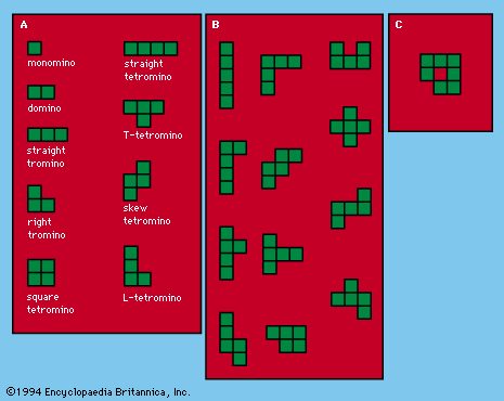
The word “polyomino” arrived in 1953 as a playful twist on “domino.” It describes a shape made of equal-sized squares joined edge-to-edge. You can’t lift a corner without breaking the connection. Simpler versions are easy to visualize. But the real fun starts with pentominoes.

There are exactly twelve unique pentomino shapes. Asymmetrical pieces don’t get double-counted if you flip them over. They are still just one type.

Mathematicians have struggled to find a general formula for the number of distinct polyominoes based on square count. We know the numbers for specific orders, though. There are 35 hexominoes. There are 108 heptominoes, assuming you count the weird one with a hole in the middle.

Can You Fit Them All?

Puzzles involving polyominoes fall under combinatorial geometry. The goal is usually to fit pieces into specific shapes or cover a board without gaps.

Take the 35 hexominoes. Together, they cover 210 squares. You might think you could arrange them into a simple rectangle. The math suggests options like 3 by 70, 5 by 42, or 14 by 15. But it doesn’t work. No such rectangle can be formed.

What about the twelve pentominoes plus one square tetromino? Can they fill an 8×8 checkerboard?

Yes. This problem dates back to around 1935. We don’t know the total number of solutions, but estimates put it at least 1,000. A computer crunch in 1958 proved there are 65 solutions where the single square piece sits exactly in the center.

Soma Cubes

The concept extends into three dimensions. Just as polyominoes are flat shapes, Soma cubes are 3D structures. They break down into seven irregular pieces. Each piece is made of four or five cubes joined face-to-face.

Benjamin Seymour Wright, a physicist, and John Horton Conway, a mathematician, helped popularize the puzzle in the 1950s. The challenge is simple. Take the seven pieces. Build a 3x3x3 cube.

There are 240 distinct ways to solve it. If you ignore rotations and reflections, the number drops. But the variety is staggering. The Soma cube is essentially the 3D equivalent of the pentomino problem. It requires spatial reasoning rather than just flat geometry.

“The number of distinct polyominoes of any order is a function of the number of squares in each, but, as yet, no general formula has been found.”

Pentominoes and hexominoes remain popular because they are deceptively simple. They look like toys. They act like complex algorithms.

The hole in that heptomino still bothers some purists. It breaks the “simply connected” rule. But it exists. And it counts.

Do you prefer the flat challenge of the 8×8 board or the 3D twist of the Soma cube? The computer found 65

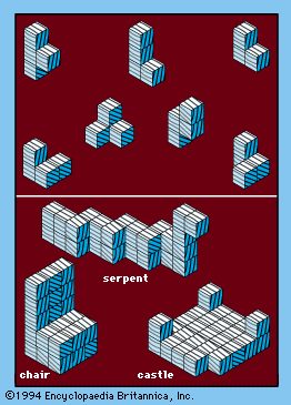
The Geometry of Play

Denmark’s Piet Hein didn’t just invent hex and tac-tix. He stumbled onto something weirder. You take three or four congruent cubes. Join them at their faces. The resulting irregular shapes? There are exactly seven of them. Mathematicians call them Soma Cubes. Put them back together, and they form a larger, perfect cube. It’s a fact that defies easy explanation.

The fifth and sixth shapes are mirror images. No two pieces are alike. Yet, these seven chunks—27 unit cubes total—snap back into a 3x3x3 block in more than 230 essentially different ways.

The variety of interesting structures possible seems endless.

You can build a sofa. A chair. A castle. A tunnel. A pyramid. Just by rearranging the basic pieces. As a pastime, the Soma Cubes are addictive. People solve them mentally with experience. Psychologists have found a rough correlation between solving speed and general intelligence. There are anomalies at both ends of the spectrum, sure. But players don’t stop. They keep building.

Colored Squares and Cubes

Then there are the colored puzzles. Tiles. Cubes. Edges that must match.

Consider the 4×6 rectangle puzzle. You have 24 three-color patterns from subdivided square tiles. Arrange them so touching edges are the same color. And the entire border? One single color. Simple in description. Hard in practice.

More famous is the 30 Colored Cubes Puzzle. Paint six colors on the faces of cubes. There are 2,226 total combinations. Select only those with all six colors. You get 30 distinct cubes. Two cubes are “different” if you can’t place them side-by-side so all corresponding faces match.

These appeared commercially under names like the Mayblox Puzzle, the Tantalizer, and the Katzenjammer. But the real shift came with Instant Insanity.

Four cubes. White, red, green, blue. Assemble them into a 1x1x4 prism. Each of the four long faces must show all four colors. Each cube has 24 orientations. That leaves 82,944 possible arrangements. Only two work.

Then, Instant Insanity was swallowed by something bigger.

The Rise of the Rubik’s Cube

Ernő Rubik patented it in Hungary in 1975. Terutoshi Ishigi filed in Japan in 1976. The Rubik’s Cube was born.

It looks like 27 smaller cubes. In the solved state, each of the six faces is a solid color. Commercial versions use an internal pivot system. Rotate a layer. The cubelets scramble.

The challenge is restoring order. The number of reachable states is more than 10^19. A thriving literature emerged quickly. Mathematicians used group theory to map systematic solutions. The puzzle wasn’t just a toy. It was a mathematical beast.

Nim and Similar Games

Nim is older than records show. Its origin is obscure. But it lends itself to hard math.

Take any number of objects. Divide them into piles. Two players take turns. Pick a pile. Remove one or all objects. The player who takes the last object wins.

Every position is either “safe” or “unsafe.”
If you leave your opponent in an unsafe position, you can force a win.
If you leave them in a safe position, any move you make hands them the advantage.

How do you know which is which? Binary notation. Add up the columns of objects in each pile. If every column adds to zero or an even number, the position is safe.

Example: Three piles with 4, 9, and 15 objects.

The calculation looks like this:

4: 0 1 0 0
9: 1 0 0 1
15: 1 1 1 1

---

Sum:2 2 1 0

Two is even. Two is even. One is odd. One is even.

The odd column breaks the safety. The position is unsafe.

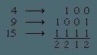
The logic of game theory doesn’t stop at simple arithmetic. If an unsafe position remains, a skilled player will always maneuver to shift the board into a safe state. It is a matter of survival in the game’s abstract architecture.

Consider a variation with just two piles. You can take objects from either pile. Or both. But if you take from both, you must take the same number from each. The person who takes the last counter wins.

Games like Nim demand a specific mental agility. You need to translate decimal numbers into binary and back again. It is not intuitive for most humans. It is, however, perfect for machines. Digital computers run on binary. They speak it natively. Because of this, it is possible to program a computer to play a perfect game.

Edward Uhler Condon and an associate invented just such a machine. The automatic Nimatron. It made its debut at the New York World’s Fair in 1940. A beating human player by sheer calculation.

Global Counting Games

These games are not isolated curiosities. They are played worldwide. Take the game of pebbles, also known as the game of odds. Two people start with an odd number of pebbles in a single pile. They take turns drawing one, two, or three pebbles. When the pile is empty, the player holding an odd count wins.

Predecessors to these exist. They are older. The mancala games. Players distribute pebbles, seeds, or counters into rows of holes. The rules vary. They have been played for centuries in Africa and Asia. The mechanics are simple. The strategy is deep.

Problems of Logical Inference

Many puzzles do not involve numbers. They involve geometry rarely, if at all. They call for deductive inference based on logical relationships.

Do not confuse these with riddles. Riddles rely on ambiguity. They use wordplay. They intend to catch the unwary. Logical puzzles have no standard procedure. There is no generalized pattern for their solution. You solve them by trial and error.

The guessing is not haphazard. The given facts—usually minimal—suggest several hypotheses. You reject the inconsistent ones. Through substitution and elimination, the solution emerges. Techniques of logic help. But success depends on ingenuity. An elusive capacity.

Logic problems are grouped here for convenience.

The Brakeman, the Fireman, and the Engineer

This is a classic. The version from Oswald Jacoby and William Benson’s Mathematics for Pleasure (1962) remains definitive.

The names of the brakeman, fireman, and engineer were Smith, Jones, and Robinson. Not necessarily in that order. Three passengers shared these names. To avoid confusion, we call them Mr. Smith, Mr. Jones, and Mr. Robinson.

Here are the facts:
– Mr. Robinson lived in Detroit.
– The brakeman lived halfway between Chicago and Detroit.
– Mr. Jones earned exactly $2,000 per year.
– Smith beat the fireman at billiards.
– The brakeman’s next-door neighbor (a passenger) earned exactly three times as much as the brakeman.
– The passenger who lived in Chicago had the same name as the brakeman.

What was the name of the engineer?

The solution requires stripping away impossibilities. You cannot assume the names match the roles directly. You have to map the geography to the income. You have to link the billiard victory to the profession. It is a tight knot of constraints.

Overlapping Groups

This category deals with sets. The high-school language club problem is typical.

Among the members:
– 21 studied French.
– 20 studied German.
– 26 studied Spanish.
– 12 studied both French and Spanish.
– 10 studied both French and German.
– 9 studied both Spanish and German.
– 3 studied French, Spanish, and German.

How many club members were there? How many studied only one language?

The numbers overlap. You cannot just add them up. You have to account for the intersections. The Venn diagram logic is implicit here. You subtract the overlaps from the totals. Then you adjust for the triple overlap. The answer is not in the sum. It is in the structure of the groups.

Truths and Lies

Another variety concerns the reliability of statements. Knights and knaves.

The natives of a certain island are knights or knaves. They look identical. Knights always tell the truth. Knaves always lie.

A visitor meets three natives. He asks if they are knights or knaves. The first says something inaudible. The second points to the first and says, “He says that he is a knight.” The third points to the second and says, “He lies.”

The visitor knows only one is a knave. He decides what each is.

If the first said he was a knight, he would be lying if he were a knave. Or telling the truth if he were a knight. The second native reports this statement. If the second is a knight, he reports truthfully. If he is a knave, he lies about what was said. The third calls the second a liar.

It is a chain of verification. One break in the chain reveals the liar.

A different type involves four men. One committed a crime. The police question them.

• Archie: Dave did it.
• Dave: Tony did it.
• Gus: I didn’t do it.
• Tony: Dave lied when he said I did it.

If only one statement is true, who is the guilty man? If only one statement is false, who is the guilty man?

The source is C.R. Wylie, Jr.’s 101 Puzzles in Thought and Logic (1957). Dover Publications. The paradoxes hinge on the contradiction between Dave and Tony. Dave accuses Tony. Tony says Dave lied. They cannot both be telling the truth. They cannot both be lying about the accusation itself in a way that preserves the “one truth” rule easily. You have to test each suspect. Assume Archie is guilty. Check the statements. Assume Dave is guilty. Check the statements. The truth emerges from the elimination of the impossible scenarios.

The logic holds. Or it doesn’t. You have to decide which one fits.

How the Smudged Forehead Puzzle Works

The story of the three travelers and their soot-stained faces is a classic example of pure logical deduction. Three men exit a train tunnel. Each has a smudge of soot on their forehead, but none can see their own face. They laugh at each other. Before they can check mirrors, a fellow passenger proposes a test.

Look at the other two. If you see at least one smudged forehead, raise your hand.

All three raise their hands instantly. The rule is simple: keep your hand raised until you are certain of your own status, then drop it.

After a moment, one man drops his hand. He knows he is smudged. Here is how he figured it out.

If he were clean, the other two men would only see one smudged face (each other). If a man sees only one smudged face, he thinks: “If I am clean, that man sees two clean faces. He would know his own face is smudged immediately because his hand is up. He would drop his hand right away.”

But they didn’t drop their hands. They hesitated. That hesitation proved to our observant traveler that the other two saw something too. They both saw his smudged face. Therefore, he knew he was dirty.

Understanding the Unexpected Hanging Paradox

The unexpected hanging paradox emerged from word of mouth in the early 1940s. It remains a tricky puzzle.

A judge tells a prisoner he will be hanged next week. The hanging will happen at noon on one day. The prisoner will not know it is coming until the morning of that day.

The prisoner argues the sentence is impossible. He starts with the last day: Saturday. If he is alive on Friday afternoon, he knows the hanging must be on Saturday. But that means he knew it in advance. This breaks the judge’s rule. So Saturday is out.

By the same logic, Friday becomes impossible too. If he survives Thursday, and Saturday is ruled out, Friday becomes the only option. He would know it again.

He works backward through the week. Monday, Tuesday, Wednesday, Thursday, Friday, Saturday all get eliminated. The prisoner concludes he is safe.

The judge can still hang him. The paradox is subtle. A statement about a future event can be true for the judge while remaining unknown to the prisoner until the event actually happens. The prisoner’s logic fails because it assumes the prediction must be known before it happens to be valid. It doesn’t.

The History of Logical Paradoxes

These puzzles are more than just games. They touch the foundations of mathematics. They are highly amusing and often tantalizing.

The Cretan prophet Epimenides caused trouble as early as the 6th century BCE. He said, “All Cretans are liars.” Since Epimenides was a Cretan, he lied. If he lied, then not all Cretans are liars. But if he told the truth, he is a liar. It is a self-contradiction.

In 1913, mathematician P.E.B. Jourdain proposed the card paradox.
Side one: “The sentence on the other side of this card is TRUE.”
Side two: “The sentence on the other side of this card is FALSE.”
If side one is true, side two is true. But side two says side one is false. Contradiction.

Bertrand Russell added the barber paradox. The barber shaves everyone in the village who does not shave themselves. Who shaves the barber?
If he shaves himself, he shouldn’t. If he doesn’t, he must. The barber paradox hinges on a statement about a class where the object is part of that class. Russell tried to fix this with a hierarchy of logical types. It didn’t fully solve the problem. The issue sits right at the heart of philosophical mathematics.

“The entire problem lies close to the philosophical foundations of mathematics.”

These puzzles force us to look at how we define truth, knowledge, and self-reference. They don’t just entertain. They expose the cracks in our reasoning. The smudged face teaches us about shared knowledge. The hanging exposes the limits of prediction. The liar and the barber show us the dangers of self-reference.

We keep coming back to them. Not because we have all the answers. But because the questions keep changing shape.